Hello everyone! Welcome to this tutorial where we’ll explore the fascinating world of Bayesian statistics to predict football match outcomes. We will cover the essential concepts needed to construct a Bayesian model that can estimate the probability of a team winning, drawing, or losing a match.
In this tutorial, our focus will be on the mathematical foundations that underpin our football forecasting model. While we won’t delve into the code just yet, this session aims to equip you with the fundamental knowledge necessary to understand Bayesian statistics and how they can be utilized to create a model for predicting football match results.
Let’s get started on this exciting journey!
Overview of the Poisson Distribution
The Poisson distribution is commonly used to model count data, such as the number of goals scored by a team in a match. It is characterized by a single parameter \(\lambda\), which represents the average rate (mean) of occurrences (goals) within a fixed interval (a match). The probability mass function (PMF) of the Poisson distribution is:
\[P(X = x | \lambda) = \frac{\lambda^x e^{-\lambda}}{x!}\]
where:
- \(X\) is the random variable representing the number of goals.
- \(\lambda\) is the rate parameter (average number of goals).
- \(x\) is the actual observed count of goals.
Simple Example
Suppose we are modeling the number of goals scored by a particular team in MLS matches. Based on historical data, we estimate that the team scores an average of 1.5 goals per match. Here, \(\lambda = 1.5\).
Let’s calculate the probability that the team scores exactly 2 goals in a match:
Substituting \(\lambda = 1.5\) and \(x = 2\):
\[ P(X = 2 | \lambda = 1.5) = \frac{1.5^2 e^{-1.5}}{2!} = \frac{2.25 \cdot e^{-1.5}}{2} = \frac{2.25 \cdot 0.22313}{2} \approx 0.251 \]
Therefore, the probability that the team scores exactly 2 goals in a match is approximately 0.251.
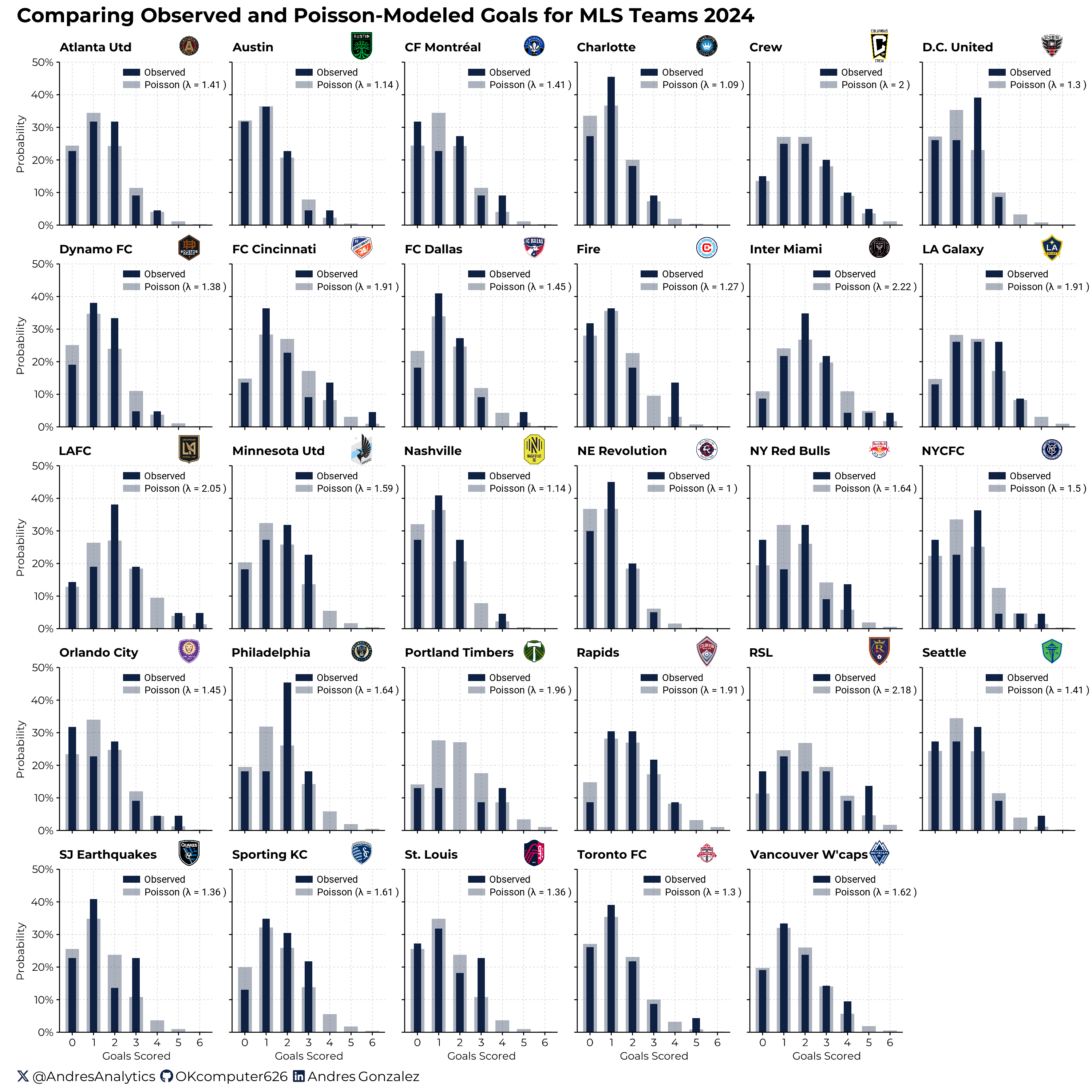
To further illustrate this, let’s look at the observed goals distribution and the expected goals distribution for various MLS teams based on their historical performance:
The above plot shows the actual observed goals distribution and the expected goals distribution (modeled using a Poisson distribution) for different MLS teams. This visual comparison helps to validate our model and understand how well the Poisson distribution can predict the number of goals scored by a team. Updating \(\lambda\) in a Bayesian framework allows us to combine prior knowledge with new data, leading to a more accurate and informed estimate. This dynamic adjustment enhances the predictive power and reliability of our Poisson model.
Introduction to the Gamma Distribution
In Bayesian statistics, the Gamma distribution is commonly used as a conjugate prior for the rate parameter (\(\lambda\)) of a Poisson distribution. This choice simplifies Bayesian updating because the posterior distribution remains within the same family. The probability density function (PDF) for the Gamma distribution is:
\[ \begin{aligned} p(\lambda | \alpha, \beta) &= \frac{\beta^\alpha \lambda^{\alpha - 1} e^{-\beta \lambda}}{\Gamma(\alpha)} \\ & \quad \text{for } \lambda > 0 \end{aligned} \]
where:
- \(\lambda\): Rate parameter for the Poisson distribution.
- \(\alpha\), \(\beta\): Shape and scale parameters of the Gamma distribution.
- \(\Gamma(\alpha)\): Gamma function evaluated at \(\alpha\).
- Mean (Expected Value): \(\mathbb{E}[\lambda] = \frac{\alpha}{\beta}\)
- Variance: \(\text{Var}(\lambda) = \frac{\alpha}{\beta^2}\)
These characteristics highlight the role of \(\alpha\) and \(\beta\) in shaping the distribution’s center (mean) and spread (variance), reflecting our confidence and the level of uncertainty in the prior assessment.
Hypothetical Football Match Example Part I
Imagine we want to estimate the number of goals that Bayesian City might score in a match against Frequentist Town.
We have reason to believe that Bayesian City, with their reasonably effective attacking lineup, can exploit the somewhat weak defense of Frequentist Town. Based on this, we assume that Bayesian City’s average goal rate is 1.92 goals per match. This goal rate reflects Bayesian City’s moderate attacking capabilities and Frequentist Town’s defensive vulnerabilities.
To incorporate this belief into our model, we set our prior parameters \(\alpha\) and \(\beta\) such that they satisfy the following equation:
\[\frac{\alpha}{\beta} = 1.92\]
- \(\alpha\) (shape parameter): Amount of prior knowledge about the team’s scoring ability.
- \(\beta\) (scale parameter): Represents how this belief spreads, analogous to an artificial sample size, influencing the prior’s certainty.
Adjusting \(\beta\) affects our confidence in \(\lambda\); a higher \(\beta\) reduces variance, indicating more confidence, whereas a lower \(\beta\) implies greater uncertainty and a wider distribution.
This explanation clarifies the Gamma distribution’s role in structuring prior beliefs and managing uncertainty in Bayesian inference for football match predictions.
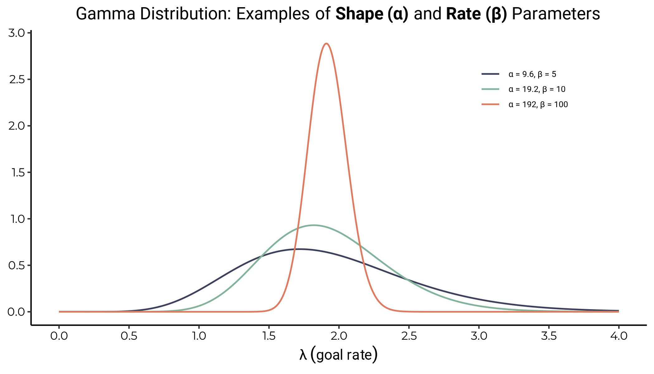
Different combinations of the shape (\(\alpha\)) and rate (\(\beta\)) parameters of the Gamma distribution, each maintaining an expected mean value of 1.92, demonstrate varying degrees of spread and height. As \(\alpha\) and \(\beta\) increase proportionally, the distribution becomes narrower and more peaked, indicating greater confidence and reduced variability in our estimate of the goal rate \(\lambda\).
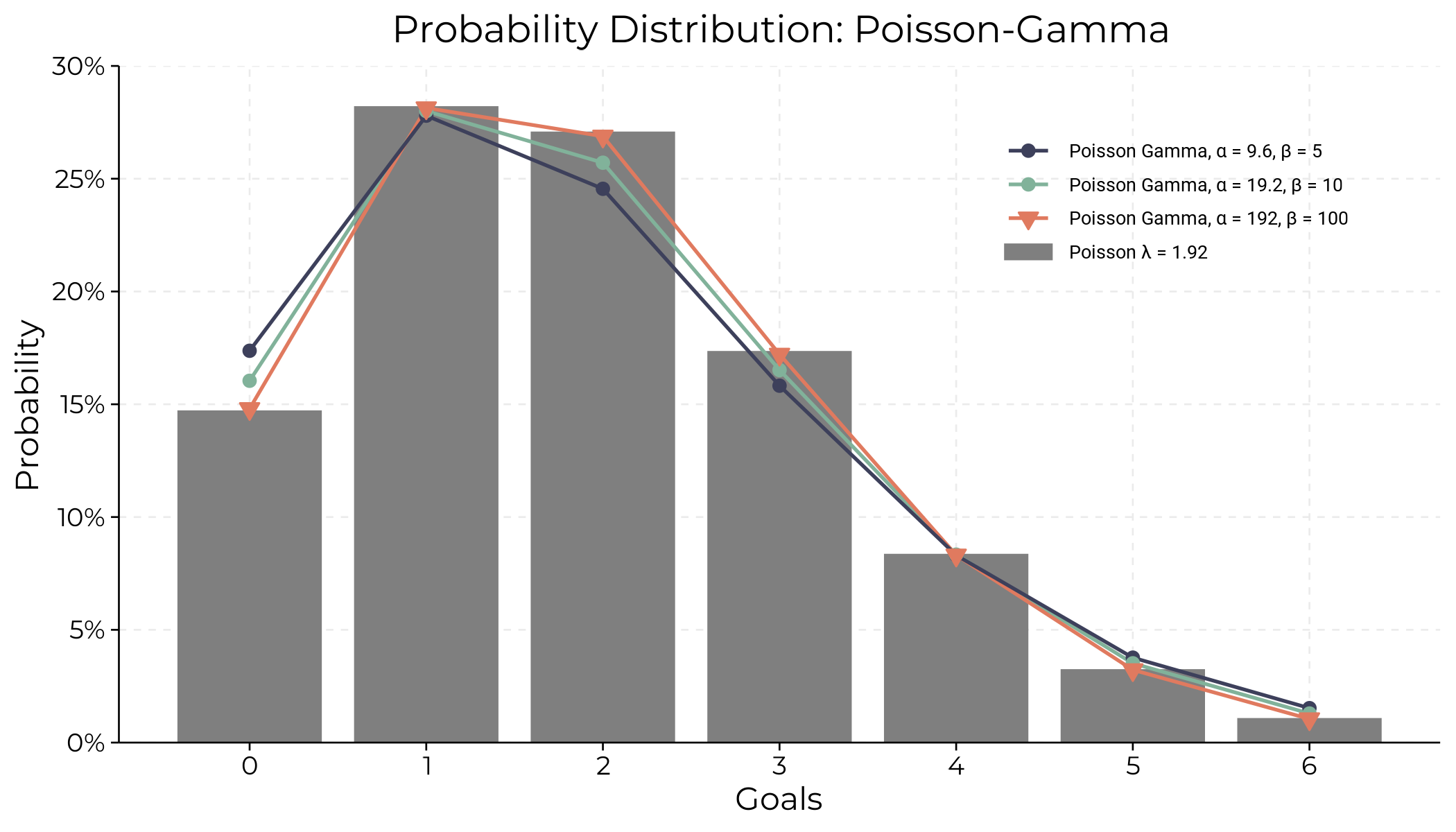
Next, we will use these Gamma priors to derive the Poisson-Gamma distribution and estimate the probability of Bayesian City scoring \(x\) goals.
Different Gamma priors impact the Poisson-Gamma distribution for Bayesian City’s goal predictions. Higher \(\alpha\) and \(\beta\) values lead to a more focused distribution, indicating greater confidence in the estimated goal rate.
Now that we have a clear understanding of the Poisson-Gamma distribution, let’s proceed to the Bayesian posterior Poisson-Gamma distribution to incorporate observed data into our predictions.
Bayesian Posterior Poisson-Gamma Distribution
The Bayesian posterior Poisson-Gamma distribution is particularly beneficial for several reasons. Firstly, it allows us to update our prior beliefs with observed data to obtain a posterior distribution that reflects both prior information and new evidence. This approach is powerful because it provides a systematic way to incorporate uncertainty from various sources, leading to more robust predictions. By accounting for both prior knowledge and observed outcomes, we can better quantify the uncertainty in our estimates and make more informed decisions.
Understanding the Bayesian Posterior Poisson-Gamma Distribution can be challenging, but it’s a powerful tool. This method allows us to update our understanding of event rates by combining prior knowledge with new data, providing a more accurate basis for making predictions about future events.
Mathematically, the posterior distribution is derived as follows:
- Prior Distribution: We start with a Gamma prior for the Poisson rate parameter \(\lambda\):
\[ \begin{aligned} p(\lambda | \alpha, \beta) &= \frac{\beta^\alpha \lambda^{\alpha - 1} e^{-\beta \lambda}}{\Gamma(\alpha)} \\ & \quad \text{for } \lambda > 0 \end{aligned} \]
- Likelihood: Given observed data, the likelihood function for a Poisson-distributed variable with observed counts \(x_1, x_2, \ldots, x_n\) is:
\[ \begin{aligned} p(x | \lambda) &= \prod_{i=1}^n \frac{e^{-\lambda} \lambda^{x_i}}{x_i!} \\ &= \frac{e^{-n\lambda} \lambda^{\sum_{i=1}^n x_i}}{\prod_{i=1}^n x_i!} \end{aligned} \]
- Posterior Distribution: Combining the prior and the likelihood using Bayes’ theorem, the posterior distribution for \(\lambda\) given the data is:
\[ \begin{aligned} p(\lambda | x) &\propto p(x | \lambda) p(\lambda | \alpha, \beta) \\ &\propto \left( \frac{e^{-n\lambda} \lambda^{\sum_{i=1}^n x_i}}{\prod_{i=1}^n x_i!} \right) \left( \frac{\beta^\alpha \lambda^{\alpha - 1} e^{-\beta \lambda}}{\Gamma(\alpha)} \right) \end{aligned} \]
Simplifying the expression by combining like terms:
\[ \begin{aligned} p(\lambda | x) &\propto e^{-n\lambda} \lambda^{\sum_{i=1}^n x_i} \lambda^{\alpha - 1} e^{-\beta \lambda} \\ &\propto \lambda^{\sum_{i=1}^n x_i + \alpha - 1} e^{-\lambda(n + \beta)} \end{aligned} \]
Since \(\prod_{i=1}^n x_i!\), \(\Gamma(\alpha)\), and \(\beta^\alpha\) are constants with respect to \(\lambda\), they can be dropped from the proportionality expression. Therefore, the posterior distribution is:
\[ \begin{aligned} p(\lambda | x) &\propto \lambda^{\sum_{i=1}^n x_i + \alpha - 1} e^{-\lambda(n + \beta)} \\ & \quad \text{for } \lambda > 0 \end{aligned} \]
The posterior distribution is a Gamma distribution with parameters:
- Shape parameter: \(\alpha' = \sum_{i=1}^n x_i + \alpha\)
- Rate parameter: \(\beta' = n + \beta\)
Expected Value (Mean) and Variance
For a Gamma distribution with shape parameter \(\alpha'\) and rate parameter \(\beta'\):
- Mean (Expected Value): \(\mathbb{E}[\lambda | x] = \frac{\alpha'}{\beta'} = \frac{\sum_{i=1}^n x_i + \alpha}{n + \beta}\)
- Variance: \(\text{Var}[\lambda | x] = \frac{\alpha'}{\beta'^2} = \frac{\sum_{i=1}^n x_i + \alpha}{(n + \beta)^2}\)
Cool, right?
Now, let’s take this mathematical framework and apply it to real football match data to predict Bayesian City’s goal-scoring rate. By incorporating our prior beliefs with actual match data, we can refine our estimates and reduce uncertainty.
Applying the Bayesian Framework
Hypothetical Football Match Example Part II
Let’s say we are interested in predicting the number of goals that Bayesian City will score in an upcoming match against Frequentist Town. Here’s how we can use the Bayesian framework to make our prediction.
In Part I, we established our prior beliefs using the Gamma distribution with parameters \(\alpha\) and \(\beta\) that reflect our prior knowledge of Bayesian City’s average goal rate of 1.92 goals per match. The prior parameters used were:
- \(\alpha = 9.6\), \(\beta = 5\)
- \(\alpha = 19.2\), \(\beta = 10\)
- \(\alpha = 192\), \(\beta = 100\)
To make a prediction, we need to update this prior distribution with observed data from previous matches. Suppose we have observed the following number of goals scored by Bayesian City in their last eight matches: 2, 1, 3, 0, 2, 2, 1, 1. We will use this data to update our prior distribution and obtain the posterior distribution.
Using the prior parameters \(\alpha = 9.6\) and \(\beta = 5\), and the observed data of 12 goals over 8 matches, the posterior distribution is a Gamma distribution with updated parameters:
\[ p(\lambda | x) \sim \text{Gamma}(\alpha', \beta') \]
where
\[ \alpha' = \alpha + \sum_{i=1}^{n} x_i \quad \text{and} \quad \beta' = \beta + n \]
In this case:
\[ \alpha' = 9.6 + 12 = 21.6 \quad \text{and} \quad \beta' = 5 + 8 = 13 \]
This distribution represents our updated belief about the goal rate \(\lambda\) after incorporating the observed data.
To predict the number of goals Bayesian City will score in the next match, we use the posterior predictive distribution. This is a Poisson distribution with the mean equal to the expected value of the posterior Gamma distribution:
\[ \mathbb{E}[\lambda | x] = \frac{\alpha'}{\beta'} \]
Therefore, the number of goals Bayesian City is expected to score in the next match follows a Poisson distribution with a mean of approximately:
\[ \mathbb{E}[\lambda | x] = \frac{21.6}{13} \approx 1.66 \]
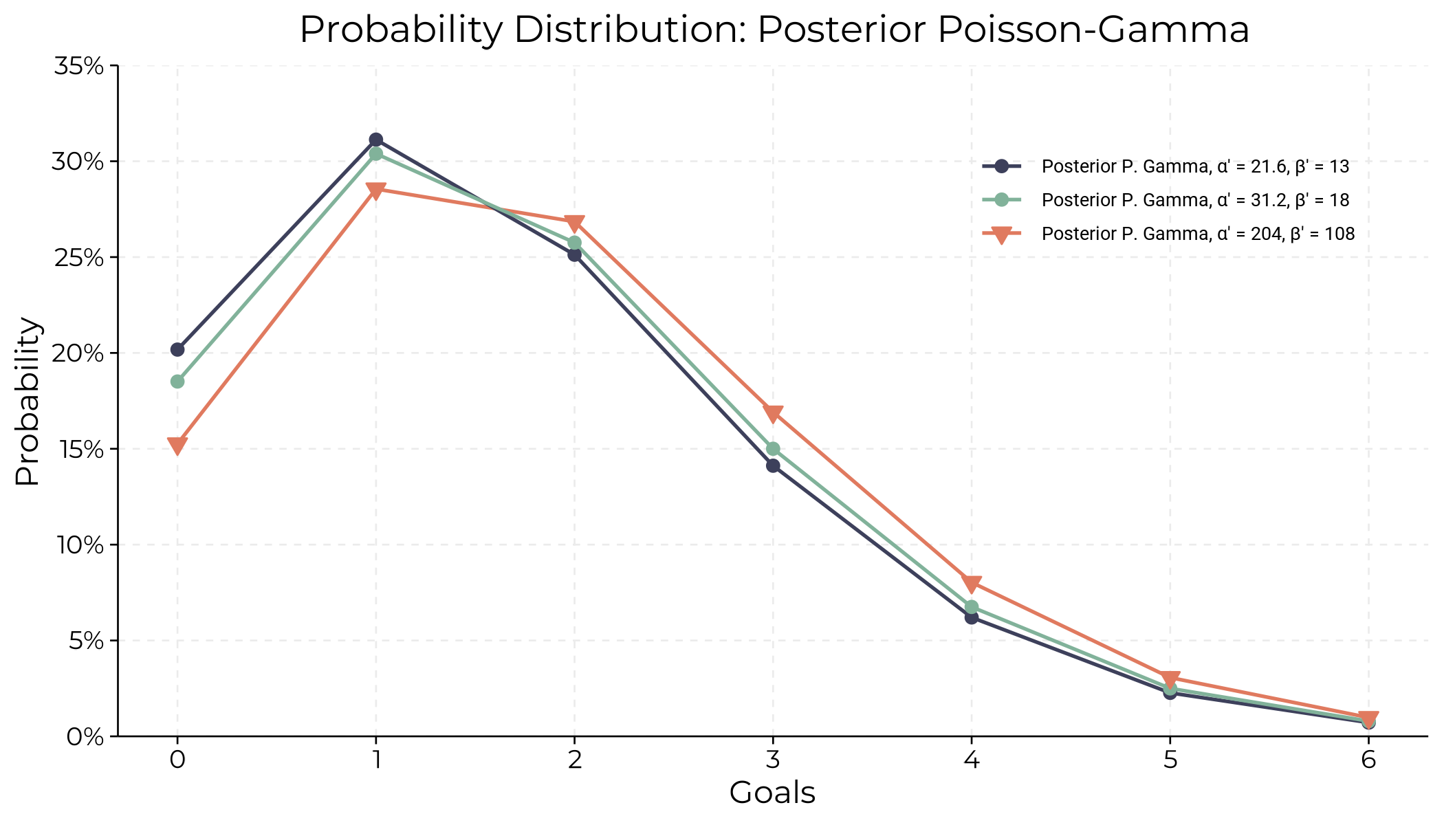
Below is the plot of the posterior Poisson-Gamma distribution for Bayesian City’s goal predictions, illustrating the probabilities of scoring different numbers of goals based on the posterior parameters:
Conclusion
By following these steps, we’ve used the Bayesian framework to update our prior beliefs with observed data and predict the number of goals Bayesian City will score in their next match. This method is a cool way to combine both our prior knowledge and new evidence in our predictions.
From our updated posterior distribution, we expect Bayesian City to score around 1.66 goals in the next match. This prediction is based on the observed data and the prior information we had about the team’s goal-scoring ability. The Bayesian approach lets us continuously update our predictions as new data comes in, making our model more robust and in tune with the team’s current performance.
This method is really awesome and powerful! By learning it, you’re getting a super useful tool for making dynamic, data-driven predictions. Hope you all learned something valuable and enjoyed working with Bayesian statistics!😎


