# Load necessary packages using pacman for easier dependency management
pacman::p_load(
  tidyverse,   # Collection of R packages for data science (ggplot2, dplyr, etc.)
  showtext,    # Enables custom fonts for ggplot2
  ggtext,      # Adds rich text formatting to ggplot2
  skimr,       # Provides summary statistics in a readable format
  janitor,     # Cleans and formats column names for consistency
  shadowtext,  # Adds text with shadows in ggplot2 for better readability
  glue         # Provides a more readable way to concatenate and format strings
)

# Add Google fonts
font_add_google("Roboto Condensed", family = "Roboto")
font_add("Simpsons", regular = here::here("fonts/Simpsons.otf"))

# Add local font
font_add("Font Awesome 6 Brands", here::here("fonts/otfs/Font Awesome 6 Brands-Regular-400.otf"))

# Automatically enable the use of showtext for all plots
showtext_auto()

# Set DPI for high-resolution text rendering
showtext_opts(dpi = 300)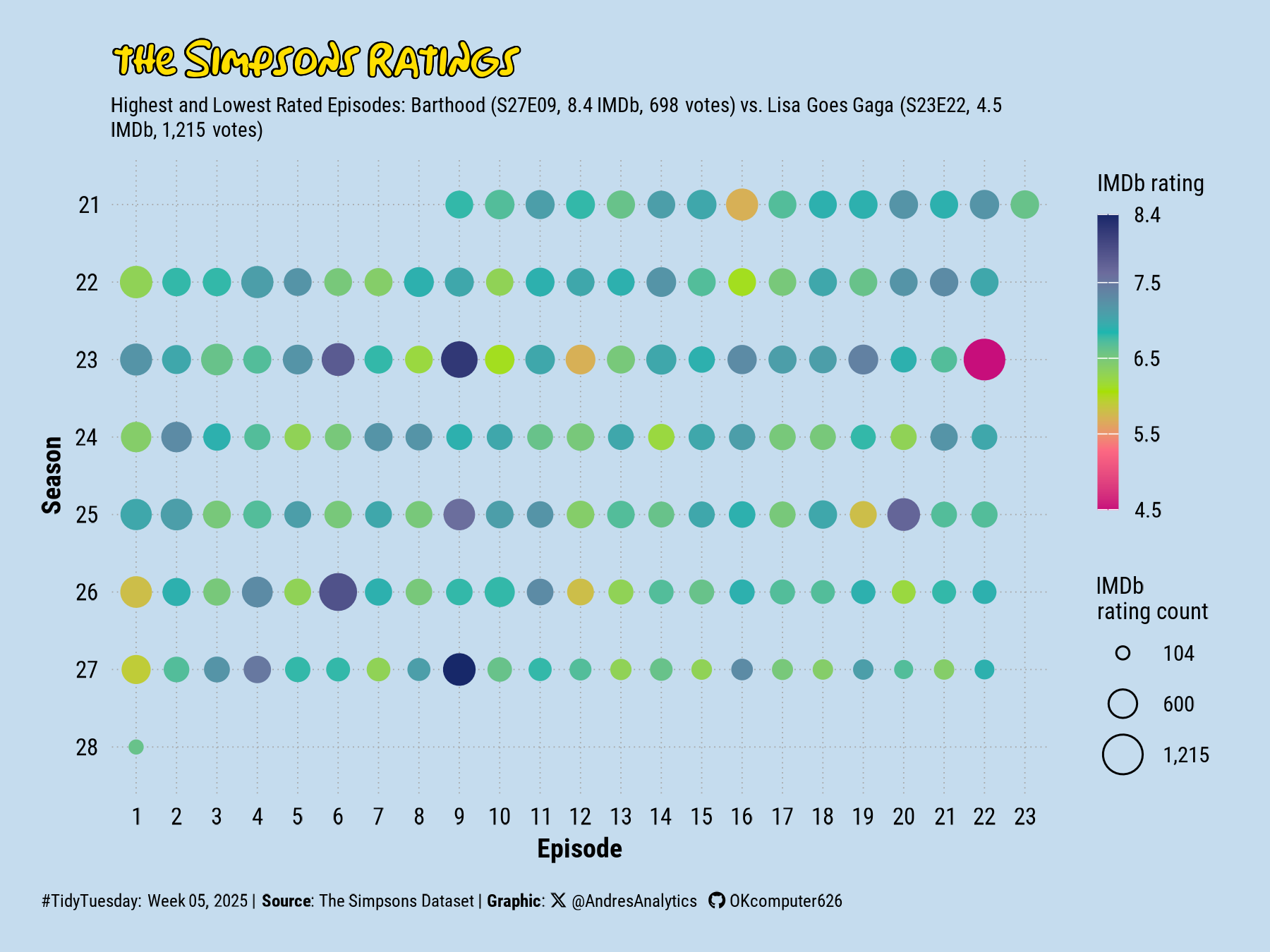
How This Graphic Was Made
1. 📦 Load Packages & Setup
2. 📖 Read in the Data
# Load the TidyTuesday data
tuesdata <- tidytuesdayR::tt_load(2025, week = 5)

characters <- tuesdata$simpsons_characters %>% clean_names()
episodes <- tuesdata$simpsons_episodes %>% clean_names()
locations <- tuesdata$simpsons_locations %>% clean_names()
script_lines <- tuesdata$simpsons_script_lines %>% clean_names()

tidytuesdayR::readme(tuesdata)  # Display dataset documentation
rm(tuesdata)  # Remove raw data object to free up memory
3. 🕵️ Examine the Data
# Preview the structure of each dataset using glimpse()
glimpse(characters)
glimpse(episodes)
glimpse(locations)
glimpse(script_lines)
4. 🤼 Wrangle Data
# Select the episode with the lowest IMDb rating
episodes %>%
  slice_min(imdb_rating) %>%
  select(imdb_rating, imdb_votes, number_in_season, season, title)

# Select the episode with the highest IMDb rating
episodes %>%
  slice_max(imdb_rating) %>%
  select(imdb_rating, imdb_votes, number_in_season, season, title)

# Select the episode with the fewest IMDb votes
episodes %>%
  slice_min(imdb_votes) %>%
  select(imdb_votes)

# Select the episode with the most IMDb votes
episodes %>%
  slice_max(imdb_votes) %>%
  select(imdb_votes)

# Remove episodes with missing IMDb ratings
episodes_clean <- episodes %>%
  drop_na(imdb_rating)

# Count the number of episodes per season
episodes_clean %>%
  group_by(season) %>%
  count(season)
5. 🔤 Text
title <- "the Simpsons Ratings"
st <- "Highest and Lowest Rated Episodes: Barthood (S27E09, 8.4 IMDb, 698 votes) vs. Lisa Goes Gaga (S23E22, 4.5 IMDb, 1,215 votes)"

# Create a social media caption with customized colors and font for consistency in visualization
social <- andresutils::social_caption(font_family = "Roboto", icon_color = "black", bg_color = "#C5DCEE")

# Construct the final plot caption by combining TidyTuesday details, data source, and the social caption
cap <- paste0(
  "#TidyTuesday: Week 05, 2025 | **Source**: The Simpsons Dataset | **Graphic**: ", social
)
6. 📊 Plot
# Create a scatter plot visualizing IMDb ratings and votes for each episode
p <- episodes_clean %>%
  ggplot(aes(x = factor(number_in_season), y = fct_rev(factor(season)))) +
  geom_point(aes(color = imdb_rating, size = imdb_votes)) +
  scale_color_gradientn(colors = LaCroixColoR::lacroix_palette("PassionFruit", type = "continuous"), breaks = c(4.5, 5.5, 6.5, 7.5, 8.4)) +
  scale_size_area(breaks = c(104, 600, 1215), label = scales::comma) +
  guides(color = guide_colorbar(barheight = unit(7, "lines"),
                                barwidth = unit(0.5, "lines"),
                                order = 1,
                                theme = theme(
                                  legend.title = element_text(margin = margin(b = 7))
                                )),
         size = guide_legend(override.aes = list(shape = 21))) +
  labs(x = "Episode",
       y = "Season",
       title = title,
       subtitle = st,
       caption = cap,
       color = "IMDb rating", size = "IMDb\nrating count") +
  theme_minimal(base_family = "Roboto") +
  theme(
    plot.title = element_shadowtext(family = "Simpsons", face = "bold", bg.r = 0.05, size = 14, color = "#FFDF00", margin = margin(b = 20), hjust = 1.15),
    plot.subtitle = element_textbox_simple(size = 7, margin = margin(b = 10), lineheight = 1.2),
    plot.background = element_rect(fill = "#C5DCEE", color = NA),
    axis.text = element_text(color = "black", size = 8),
    axis.title.x=element_text(color = "black", size = 9, face = "bold", margin = margin(t = 3)),
    axis.title.y=element_text(color = "black", size = 9, face = "bold"),
    plot.margin = margin(0.5, 0.5, 0.5, 0.5, unit = "cm"),
    panel.grid = element_line(linetype = "dotted", color = "grey65", size = 0.2),
    legend.title = element_text(size = 8, margin = margin(b = 2)),
    legend.text = element_text(size = 7.5),
    plot.caption.position = "plot",
    plot.caption = element_markdown(size = 6, hjust = 0, margin = margin(t = 10))
  )
7. 💾 Save
# Save plot with dimensions
andresutils::save_plot(p, type = "tidytuesday", year = 2025, week = 5, width = 6, height = 4.5)
8. 🚀 GitHub Repository
TipExpand for GitHub Repo
The complete code for this analysis is available in tt_05_2025.qmd.
For the full repository, click here.
Citation
For attribution, please cite this work as:
Gonzalez, Andres. 2025. “The Simpsons Dataset.” February
12, 2025. https://andresgonzalezstats.com/visualization/TidyTuesday/2025/Week_05/tt_05_2025.html.