# Load necessary packages using pacman for easier dependency management
pacman::p_load(
  tidyverse,   # Collection of R packages for data science, includes ggplot2 (visualization), dplyr (data manipulation), readr (data import)
  showtext,    # Enables custom fonts in ggplot2, allowing for enhanced typography in plots
  ggtext,      # Adds support for Markdown and HTML formatting in ggplot2 text elements (e.g., bold, italic, colored text)
  skimr,       # Provides detailed summary statistics in a readable and concise format for data exploration
  glue,        # Constructs strings efficiently using variable interpolation
  janitor,     # Simplifies data cleaning (e.g., renaming columns, removing duplicates, formatting variable names)
  paletteer,   # Provides access to a wide range of color palettes for consistent and visually appealing plots
  cowplot      # Enhances ggplot2 with better layout and annotation options, useful for combining multiple plots
)

# Add Google fonts
font_add_google("Oswald", family = "Oswald")
font <- "Oswald"

# Add local font
font_add("Font Awesome 6 Brands", here::here("fonts/otfs/Font Awesome 6 Brands-Regular-400.otf"))

# Automatically enable the use of showtext for all plots
showtext_auto()

# Set DPI for high-resolution text rendering
showtext_opts(dpi = 300)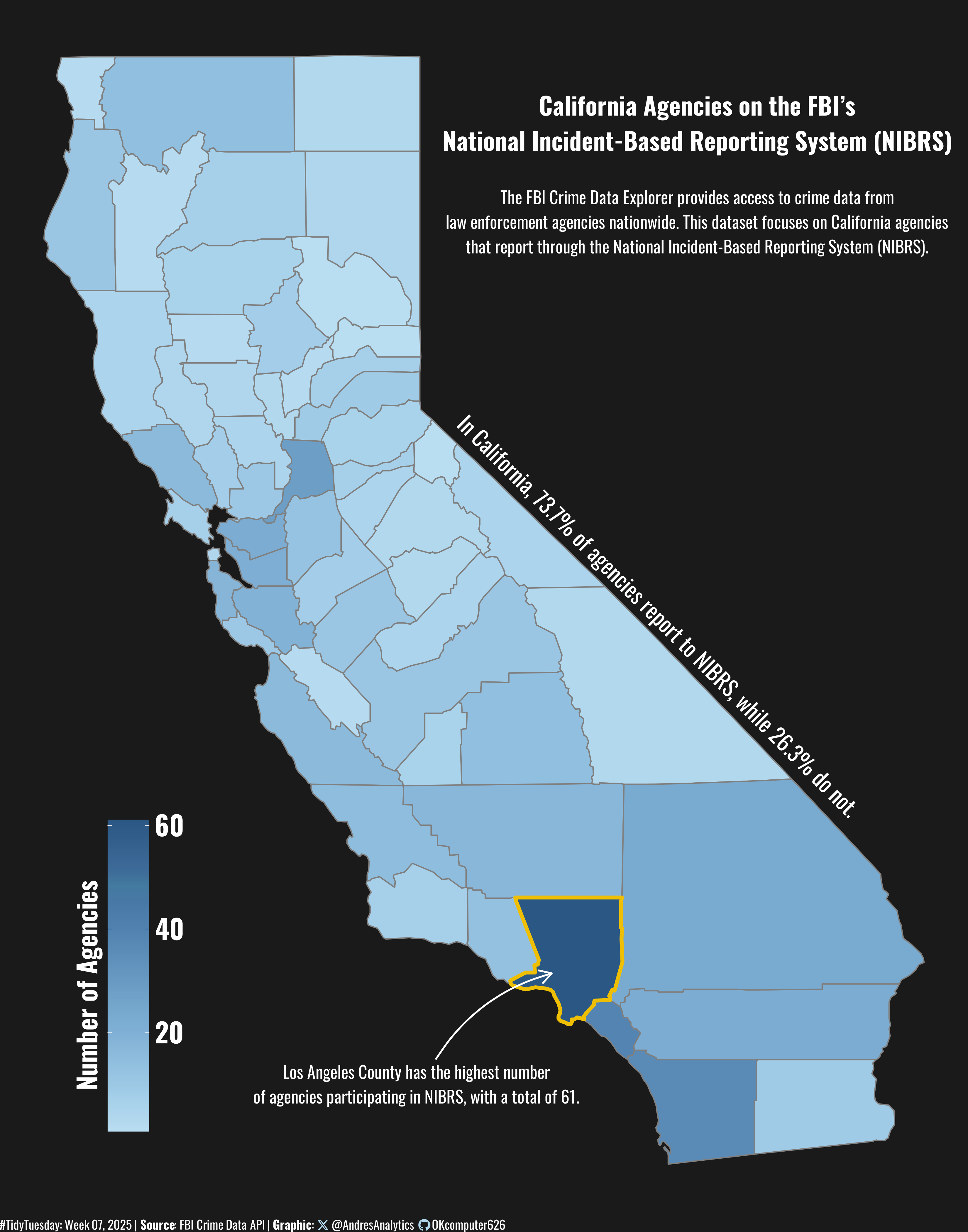
How This Graphic Was Made
1. 📦 Load Packages & Setup
2. 📖 Read in the Data
# Load the TidyTuesday dataset for Week 07 of 2025
tuesdata <- tidytuesdayR::tt_load(2025, week = 07)

# Extract and clean column names in the agencies dataset
agencies <- tuesdata$agencies %>%
  clean_names()

# Display dataset information from TidyTuesday
tidytuesdayR::readme(tuesdata)

# Remove the original loaded list to free memory
rm(tuesdata)
3. 🕵️ Examine the Data
# Display the structure of the agencies dataset, including column types and sample values
glimpse(agencies)

# Generate a detailed summary of the agencies dataset, including distribution and missing values
skim(agencies)
4. 🤼 Wrangle Data
# Get California county map data
ca_counties <- subset(map_data("county"), region == "california")

# Filter agencies for California and format county names
california <- agencies %>%
  filter(state_abbr == "CA") %>%
  mutate(county = str_to_lower(county)) %>%
  group_by(county, is_nibrs) %>%
  count(is_nibrs) %>%
  ungroup()

# Calculate the percentage of agencies reporting to NIBRS in California
perc <- california %>%
  group_by(is_nibrs) %>%
  summarise(count = sum(n)) %>%
  mutate(proportion = round(count / sum(count) * 100, 1)) %>%
  ungroup() %>%
  pull(proportion)

# Merge California county map data with agency data
california <- ca_counties %>%
  left_join(california, by = join_by(subregion == county))

# Extract data for Los Angeles County
los_angeles <- california %>%
  filter(subregion == "los angeles")
5. 🔤 Text
# Define the main title for the visualization
title <- "California Agencies on the FBI’s\nNational Incident-Based Reporting System (NIBRS)"

# Create a short description of the dataset focus
st <- "The FBI Crime Data Explorer provides access to crime data from\nlaw enforcement agencies nationwide. This dataset focuses on California agencies\nthat report through the National Incident-Based Reporting System (NIBRS)."

# Highlight key insight about agency participation in Los Angeles County
text <- "Los Angeles County has the highest number\nof agencies participating in NIBRS, with a total of 61."

# Generate the formatted text
cal_perc <- glue("In California, {perc[2]}% of agencies report to NIBRS, while {perc[1]}% do not.")

# Generate a social media caption with custom colors and font styling
social <- andresutils::social_caption(font_family = font, icon_color = "#b2d8ee", bg_color = "gray10", font_color = "white")

# Construct the final plot caption with TidyTuesday details, data source, and social caption
cap <- paste0(
  "#TidyTuesday: Week 07, 2025 | **Source**: FBI Crime Data API | **Graphic**: ", social
)
6. 📊 Plot
# Create a base map of California showing NIBRS-participating agencies
p <- california %>%
  filter(is_nibrs == "TRUE") %>%
  ggplot() +
  geom_polygon(aes(x = long, y = lat, group = group, fill = n), color = "gray50") +
  geom_polygon(data = los_angeles, aes(x = long, y = lat, group = group), color = "#EFBF04", fill = NA, size = 1.5) +
  scale_fill_paletteer_c("ggthemes::Blue") +
  labs(caption = cap) +
  theme_void() +
  theme(
    legend.position = c(0.15, 0.2),
    legend.key.width = unit(1.2, "cm"),
    legend.key.height = unit(1.8, "cm"),
    legend.title = element_blank(),
    legend.text = element_text(color="white", size = 22, family = font, face = "bold"),
    plot.background = element_rect(fill = "gray10", color = "transparent"),
    plot.caption = element_textbox_simple(color = "white", family = font, size = 10)
  )

# Add text, labels, and annotations to the map
p1 <- ggdraw(p) +
  draw_text(text = title, x = 0.72, y = 0.9, size = 20, color = "white", family = font, fontface = "bold") +
  draw_text(text = "Number of Agencies", color = "white", x = 0.09, y = 0.2, size = 21, family = font, fontface = "bold", angle = 90) +
  draw_text(text = text, x = 0.43, y = 0.12, color = "white", family = font) +
  annotate("curve", x = 0.45, y = 0.14, xend = 0.57, yend = 0.21, color = "white", curvature = -0.2, linewidth = 0.7, arrow = arrow(length = unit(0.4, 'cm'))) +
  draw_text(text = st, x = 0.72, y = 0.82, color = "white", family = font) +
  draw_text(text = cal_perc, x= 0.68, y = 0.5, color = "white", family = font, angle = -45, size = 18)
7. 💾 Save
# Save the plot for TidyTuesday 2025, Week 07 with specified dimensions.
andresutils::save_plot(p1, type = "tidytuesday", year = 2025, week = 7, width = 11, height = 14)
8. 🚀 GitHub Repository
TipExpand for GitHub Repo
The complete code for this analysis is available in tt_07_2025.qmd.
For the full repository, click here.
Citation
For attribution, please cite this work as:
Gonzalez, Andres. 2025. “Agencies from the FBI Crime Data.”
February 20, 2025. https://andresgonzalezstats.com/visualization/TidyTuesday/2025/Week_07/tt_07_2025.html.